London Fire Brigade
The London Fire Brigade attends a range of non-fire incidents (which we call ‘special services’). These ‘special services’ include assistance to animals that may be trapped or in distress. The data is provided from January 2009 and is updated monthly. A range of information is supplied for each incident including some location information (postcode, borough, ward), as well as the data/time of the incidents. We do not routinely record data about animal deaths or injuries.
Please note that any cost included is a notional cost calculated based on the length of time rounded up to the nearest hour spent by Pump, Aerial and FRU appliances at the incident and charged at the current Brigade hourly rate.
url <- "https://data.london.gov.uk/download/animal-rescue-incidents-attended-by-lfb/8a7d91c2-9aec-4bde-937a-3998f4717cd8/Animal%20Rescue%20incidents%20attended%20by%20LFB%20from%20Jan%202009.csv"

animal_rescue <- read_csv(url,
                          locale = locale(encoding = "CP1252")) %>%
  janitor::clean_names()


glimpse(animal_rescue)
## Rows: 7,873
## Columns: 31
## $ incident_number <dbl> 139091, 275091, 2075091, 2872091, 355309…
## $ date_time_of_call <chr> "01/01/2009 03:01", "01/01/2009 08:51", …
## $ cal_year <dbl> 2009, 2009, 2009, 2009, 2009, 2009, 2009…
## $ fin_year <chr> "2008/09", "2008/09", "2008/09", "2008/0…
## $ type_of_incident <chr> "Special Service", "Special Service", "S…
## $ pump_count <chr> "1", "1", "1", "1", "1", "1", "1", "1", …
## $ pump_hours_total <chr> "2", "1", "1", "1", "1", "1", "1", "1", …
## $ hourly_notional_cost <dbl> 255, 255, 255, 255, 255, 255, 255, 255, …
## $ incident_notional_cost <chr> "510", "255", "255", "255", "255", "255"…
## $ final_description <chr> "Redacted", "Redacted", "Redacted", "Red…
## $ animal_group_parent <chr> "Dog", "Fox", "Dog", "Horse", "Rabbit", …
## $ originof_call <chr> "Person (land line)", "Person (land line…
## $ property_type <chr> "House - single occupancy", "Railings", …
## $ property_category <chr> "Dwelling", "Outdoor Structure", "Outdoo…
## $ special_service_type_category <chr> "Other animal assistance", "Other animal…
## $ special_service_type <chr> "Animal assistance involving livestock -…
## $ ward_code <chr> "E05011467", "E05000169", "E05000558", "…
## $ ward <chr> "Crystal Palace & Upper Norwood", "Woods…
## $ borough_code <chr> "E09000008", "E09000008", "E09000029", "…
## $ borough <chr> "Croydon", "Croydon", "Sutton", "Hilling…
## $ stn_ground_name <chr> "Norbury", "Woodside", "Wallington", "Ru…
## $ uprn <chr> "NULL", "NULL", "NULL", "100021491149.00…
## $ street <chr> "Waddington Way", "Grasmere Road", "Mill…
## $ usrn <chr> "20500146.00", "NULL", "NULL", "21401484…
## $ postcode_district <chr> "SE19", "SE25", "SM5", "UB9", "RM3", "RM…
## $ easting_m <chr> "NULL", "534785", "528041", "504689", "N…
## $ northing_m <chr> "NULL", "167546", "164923", "190685", "N…
## $ easting_rounded <dbl> 532350, 534750, 528050, 504650, 554650, …
## $ northing_rounded <dbl> 170050, 167550, 164950, 190650, 192350, …
## $ latitude <chr> "NULL", "51.39095371", "51.36894086", "5…
## $ longitude <chr> "NULL", "-0.064166887", "-0.161985191", …One of the more useful things one can do with any data set is quick counts, namely to see how many observations fall within one category. For instance, if we wanted to count the number of incidents by year, we would either use group_by()... summarise() or, simply count()
animal_rescue %>%
  dplyr::group_by(cal_year) %>%
  summarise(count=n())
## # A tibble: 13 x 2
## cal_year count
## <dbl> <int>
## 1 2009 568
## 2 2010 611
## 3 2011 620
## 4 2012 603
## 5 2013 585
## 6 2014 583
## 7 2015 540
## 8 2016 604
## 9 2017 539
## 10 2018 610
## 11 2019 604
## 12 2020 758
## 13 2021 648animal_rescue %>%
count(cal_year, name="count")## # A tibble: 13 x 2
## cal_year count
## <dbl> <int>
## 1 2009 568
## 2 2010 611
## 3 2011 620
## 4 2012 603
## 5 2013 585
## 6 2014 583
## 7 2015 540
## 8 2016 604
## 9 2017 539
## 10 2018 610
## 11 2019 604
## 12 2020 758
## 13 2021 648Let us try to see how many incidents we have by animal group. Again, we can do this either using group_by() and summarise(), or by using count()
animal_rescue %>%
  group_by(animal_group_parent) %>%

  #group_by and summarise will produce a new column with the count in each animal group
  summarise(count = n()) %>%

  # mutate adds a new column; here we calculate the percentage
  mutate(percent = round(100*count/sum(count),2)) %>%

  # arrange() sorts the data by percent. Since the default sorting is min to max and we would like to see it sorted
  # in descending order (max to min), we use arrange(desc())
  arrange(desc(percent))
## # A tibble: 28 x 3
## animal_group_parent count percent
## <chr> <int> <dbl>
## 1 Cat 3783 48.0
## 2 Bird 1631 20.7
## 3 Dog 1230 15.6
## 4 Fox 373 4.74
## 5 Unknown - Domestic Animal Or Pet 201 2.55
## 6 Horse 195 2.48
## 7 Deer 136 1.73
## 8 Unknown - Wild Animal 94 1.19
## 9 Squirrel 68 0.86
## 10 Unknown - Heavy Livestock Animal 50 0.64
## # … with 18 more rowsanimal_rescue %>%
#count does the same thing as group_by and summarise
# name = "count" will call the column with the counts "count" ( exciting, I know)
# and 'sort=TRUE' will sort them from max to min
count(animal_group_parent, name="count", sort=TRUE) %>%
mutate(percent = round(100*count/sum(count),2))## # A tibble: 28 x 3
## animal_group_parent count percent
## <chr> <int> <dbl>
## 1 Cat 3783 48.0
## 2 Bird 1631 20.7
## 3 Dog 1230 15.6
## 4 Fox 373 4.74
## 5 Unknown - Domestic Animal Or Pet 201 2.55
## 6 Horse 195 2.48
## 7 Deer 136 1.73
## 8 Unknown - Wild Animal 94 1.19
## 9 Squirrel 68 0.86
## 10 Unknown - Heavy Livestock Animal 50 0.64
## # … with 18 more rowsDo you see anything strange in these tables? Some animal group parents are repetitive and may also overlap giving a skewed sense of the data.
Finally, let us have a look at the notional cost for rescuing each of these animals. As the LFB says,
Please note that any cost included is a notional cost calculated based on the length of time rounded up to the nearest hour spent by Pump, Aerial and FRU appliances at the incident and charged at the current Brigade hourly rate.
There is two things we will do:
- Calculate the mean and median
incident_notional_costfor eachanimal_group_parent - Plot a boxplot to get a feel for the distribution of
incident_notional_costbyanimal_group_parent.
Before we go on, however, we need to fix incident_notional_cost as it is stored as a chr, or character, rather than a number.
# what type is variable incident_notional_cost from dataframe `animal_rescue`
typeof(animal_rescue$incident_notional_cost)
## [1] "character"# readr::parse_number() will convert any numerical values stored as characters into numbers
animal_rescue <- animal_rescue %>%
# we use mutate() to use the parse_number() function and overwrite the same variable
mutate(incident_notional_cost = parse_number(incident_notional_cost))
# incident_notional_cost from dataframe `animal_rescue` is now 'double' or numeric
typeof(animal_rescue$incident_notional_cost)## [1] "double"Now that incident_notional_cost is numeric, let us quickly calculate summary statistics for each animal group.
animal_rescue %>%

  # group by animal_group_parent
  group_by(animal_group_parent) %>%

  # filter resulting data, so each group has at least 6 observations
  filter(n()>6) %>%

  # summarise() will collapse all values into 3 values: the mean, median, and count
  # we use na.rm=TRUE to make sure we remove any NAs, or cases where we do not have the incident cos
  summarise(mean_incident_cost = mean (incident_notional_cost, na.rm=TRUE),
            median_incident_cost = median (incident_notional_cost, na.rm=TRUE),
            sd_incident_cost = sd (incident_notional_cost, na.rm=TRUE),
            min_incident_cost = min (incident_notional_cost, na.rm=TRUE),
            max_incident_cost = max (incident_notional_cost, na.rm=TRUE),
            count = n()) %>%

  # sort the resulting data in descending order. You choose whether to sort by count or mean cost.
  arrange(mean_incident_cost)
## # A tibble: 16 x 7
## animal_group_parent mean_incident_co… median_incident_… sd_incident_cost
## <chr> <dbl> <dbl> <dbl>
## 1 Rabbit 309. 326 32.2
## 2 Ferret 309. 333 39.4
## 3 Squirrel 314. 326 56.7
## 4 Hamster 315. 290 95.0
## 5 cat 324. 290 94.1
## 6 Unknown - Domestic Anim… 326. 295 116.
## 7 Cat 344. 326 160.
## 8 Bird 344. 328 134.
## 9 Dog 347. 298 168.
## 10 Snake 356. 339 105.
## 11 Fox 374. 328 205.
## 12 Unknown - Heavy Livesto… 374. 260 263.
## 13 Deer 415. 333 282.
## 14 Unknown - Wild Animal 416. 333 322.
## 15 Cow 599. 436 451.
## 16 Horse 740. 596 541.
## # … with 3 more variables: min_incident_cost <dbl>, max_incident_cost <dbl>,
## # count <int>Compare the mean and the median for each animal group. What do you think this is telling us? Anything else that stands out? Any outliers?
While for most animal groups the mean and median costs are close to each other, none represent equal mean and median. This may be essentially because mean is affected by outliers. For instance, the category ‘Horse’ has a minimum cost of 255 and maximum of 3480, therefore the mean is extremely high and differs from the median significantly. Both these measures of central tendency differ as median shows the middle value of dataset and mean is affected algebraically.
Another observation could be that for two repetitive categories “Cat” and “cat” the true mean / median cost will be when the categories are grouped together such that the sample is more representative.
Finally, let us plot a few plots that show the distribution of incident_cost for each animal group.
# base_plot
base_plot <- animal_rescue %>%
  group_by(animal_group_parent) %>%
  filter(n()>6) %>%
  ggplot(aes(x=incident_notional_cost))+
  facet_wrap(~animal_group_parent, scales = "free")+
  theme_bw()

base_plot + geom_histogram()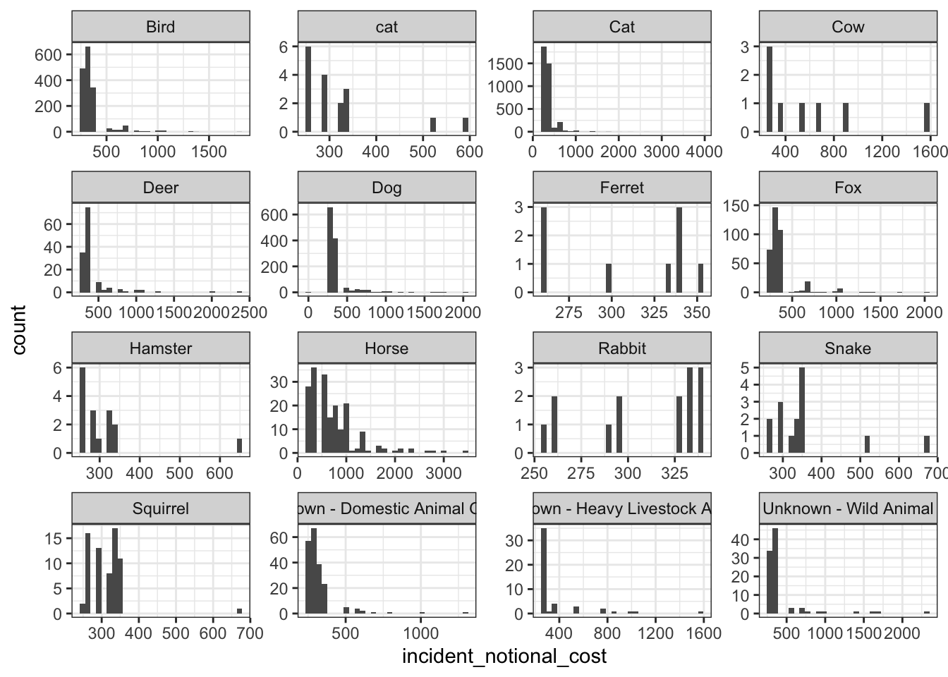
base_plot + geom_density()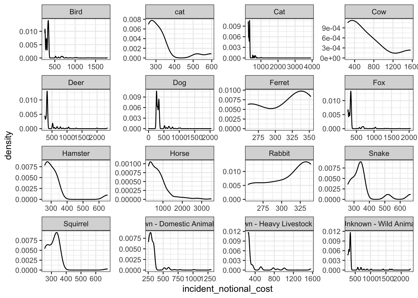
base_plot + geom_boxplot()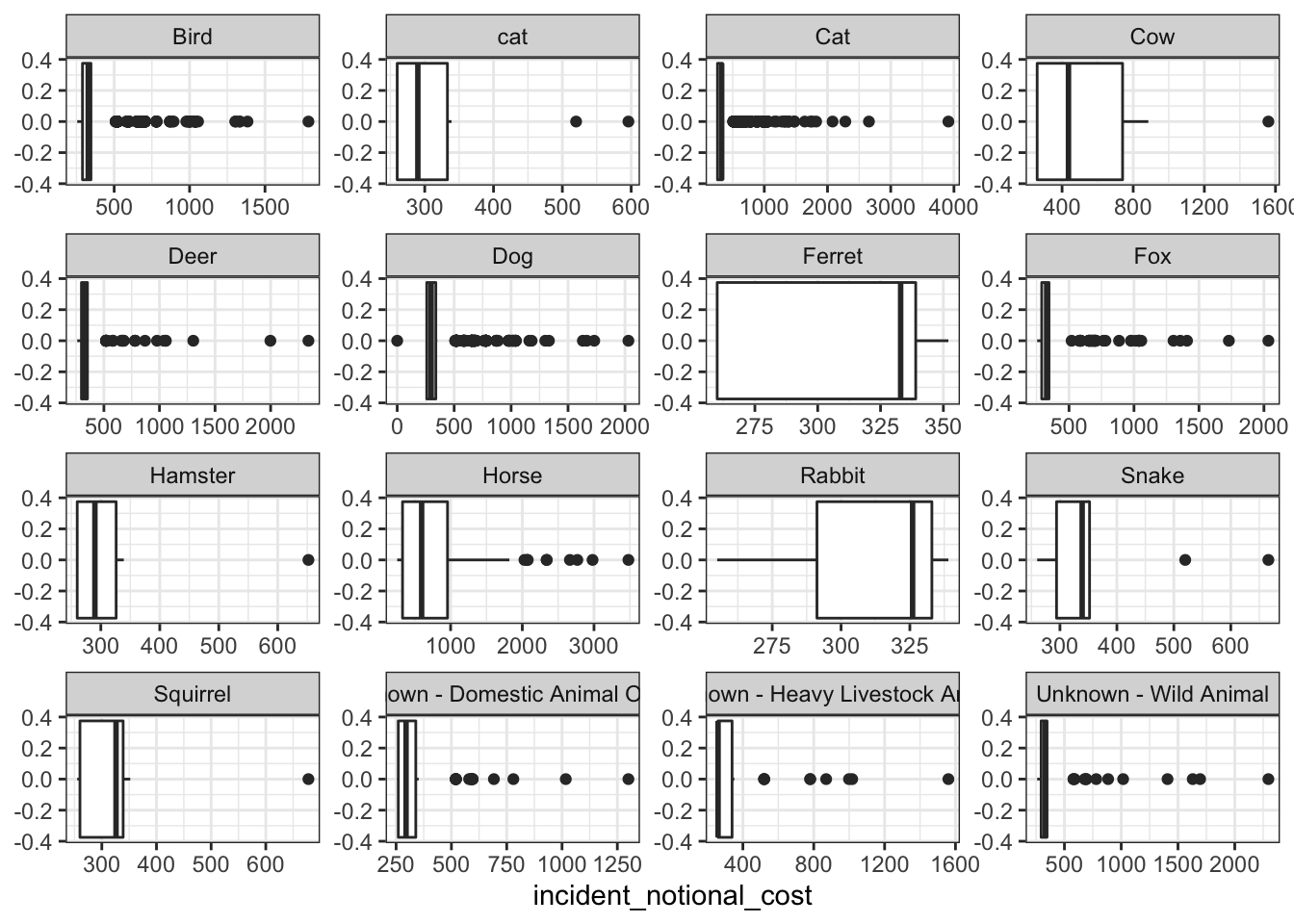
base_plot + stat_ecdf(geom = "step", pad = FALSE) +
  scale_y_continuous(labels = scales::percent)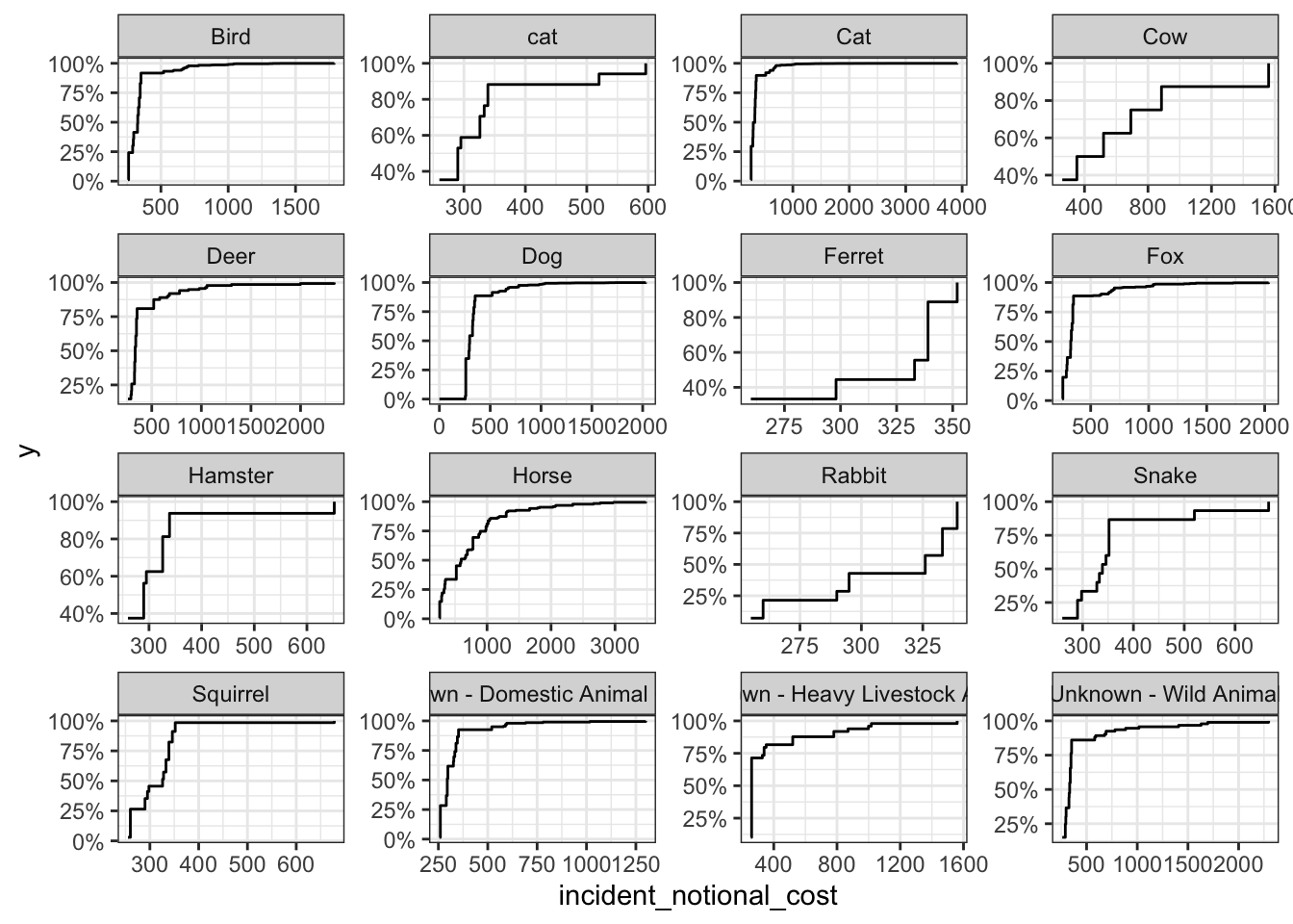
Which of these four graphs do you think best communicates the variability of the incident_notional_cost values? Also, can you please tell some sort of story (which animals are more expensive to rescue than others, the spread of values) and speculate about the differences in the patterns.
In my opinion, the box-plot best communicates the variability of the incident notional cost values. This is because it gives the interquartile range and outliers which are important metrics in this data-set. For instance, the incident notional cost for a Squirrel is represented by the box on the extreme left (250-350), however it also depicts an outlier cost of >600 which might be a particular case of serious injury.
The costs seem to be associated with size and frequency of incidents.
The most expensive to rescue of them all are horses, with extreme outliers, as the team would require heavy and highly advanced equipment owing to the size of the horse.
Cow’s have an average rescue cost of 500 and a fixed spread of values.
Squirrels, Rabbits, Hamsters and Ferrets have approximately similar spread of values and average rescue cost, could be to similar due to size and nature of injuries, due to small and fragile bodies.
Dogs, cats and deer have almost similar spread of values and average costs. These are often involved in road accidents and mishaps that require professional healthcare services. However, these often heal themselves on minor injuries therefore the costs may be not subsequently high. One of the reasons for many outliers in the plot of cats and dogs could be because these are pets and pet owners are willing to spend on advanced medical and rescue services.
Birds have a relatively short spread of cost value possibly due to defined treatment and difficulty in rescue. However, their outlying values are high due to their complex anatomy and fragility.
Finally, rescue teams and veterinary services for wild animals are specialists, providing defined treatment and may charge higher for their services. The teams would have to be well equipped to save from midst the wildlife.