Exploring IMDB Ratings Between Spielberg and Burton

IMDB ratings: Differences between directors
To explore whether the mean IMDB rating for Steven Spielberg and Tim Burton are the same or not. We calculate the confidence intervals for the mean ratings of these two directors and see they overlap.
movies <- read_csv(here::here("data", "movies.csv"))##
## ── Column specification ────────────────────────────────────────────────────────
## cols(
## title = col_character(),
## genre = col_character(),
## director = col_character(),
## year = col_double(),
## duration = col_double(),
## gross = col_double(),
## budget = col_double(),
## cast_facebook_likes = col_double(),
## votes = col_double(),
## reviews = col_double(),
## rating = col_double()
## )glimpse(movies)## Rows: 2,961
## Columns: 11
## $ title <chr> "Avatar", "Titanic", "Jurassic World", "The Avenge…
## $ genre <chr> "Action", "Drama", "Action", "Action", "Action", "…
## $ director <chr> "James Cameron", "James Cameron", "Colin Trevorrow…
## $ year <dbl> 2009, 1997, 2015, 2012, 2008, 1999, 1977, 2015, 20…
## $ duration <dbl> 178, 194, 124, 173, 152, 136, 125, 141, 164, 93, 1…
## $ gross <dbl> 760505847, 658672302, 652177271, 623279547, 533316…
## $ budget <dbl> 2.37e+08, 2.00e+08, 1.50e+08, 2.20e+08, 1.85e+08, …
## $ cast_facebook_likes <dbl> 4834, 45223, 8458, 87697, 57802, 37723, 13485, 920…
## $ votes <dbl> 886204, 793059, 418214, 995415, 1676169, 534658, 9…
## $ reviews <dbl> 3777, 2843, 1934, 2425, 5312, 3917, 1752, 1752, 35…
## $ rating <dbl> 7.9, 7.7, 7.0, 8.1, 9.0, 6.5, 8.7, 7.5, 8.5, 7.2, …burton_spielberg <- movies %>%
filter(director %in% c("Steven Spielberg", "Tim Burton")) %>%
group_by(director) %>%
summarise(mean=mean(rating),
count=n(),
t_critical = qt(0.975, count-1),
se = sd(rating)/sqrt(count),
margin_of_error = t_critical*se,
lower_ci = mean - margin_of_error,
higher_ci = mean + margin_of_error)
burton_spielberg## # A tibble: 2 x 8
## director mean count t_critical se margin_of_error lower_ci higher_ci
## <chr> <dbl> <int> <dbl> <dbl> <dbl> <dbl> <dbl>
## 1 Steven Spielb… 7.57 23 2.07 0.145 0.301 7.27 7.87
## 2 Tim Burton 6.93 16 2.13 0.187 0.399 6.53 7.33We calculate the mean, t-critical and confidence intervals for the mean ratings.
plot <- ggplot(burton_spielberg, aes(x=mean, y=reorder(director, mean), colour = director))+
  geom_errorbar(width = 0.05, aes(xmin = lower_ci, xmax = higher_ci), size = 2)+
  geom_point(aes(x=mean), size = 5)+
  geom_rect(aes(xmin = max(lower_ci), xmax = min(higher_ci), ymin = Inf, ymax = Inf),
            fill="gray", colour="gray",alpha = 0.3)+
  theme_bw() +
  geom_text(aes(x=mean, label = round(mean, digits=2)),
            size = 8, vjust = 2, color = "black")+
  geom_text(aes(x=lower_ci, label=round(lower_ci,digits=2)),
            size = 6, vjust = 2, color = "black")+
  geom_text(aes(x=higher_ci, label=round(higher_ci,digits=2)),
            size = 6, vjust = 2, colour = "black")+
  labs(title = "Do Spielberg ad Burton have the same IMDB ratings?",
       subtitle = "95% confidence intervals overlap", x="Mean IMDB Rating", y="")+
  theme(plot.title=element_text(size=12,face="bold"),
        axis.text = element_text(size=10),
        legend.position = "none")
plot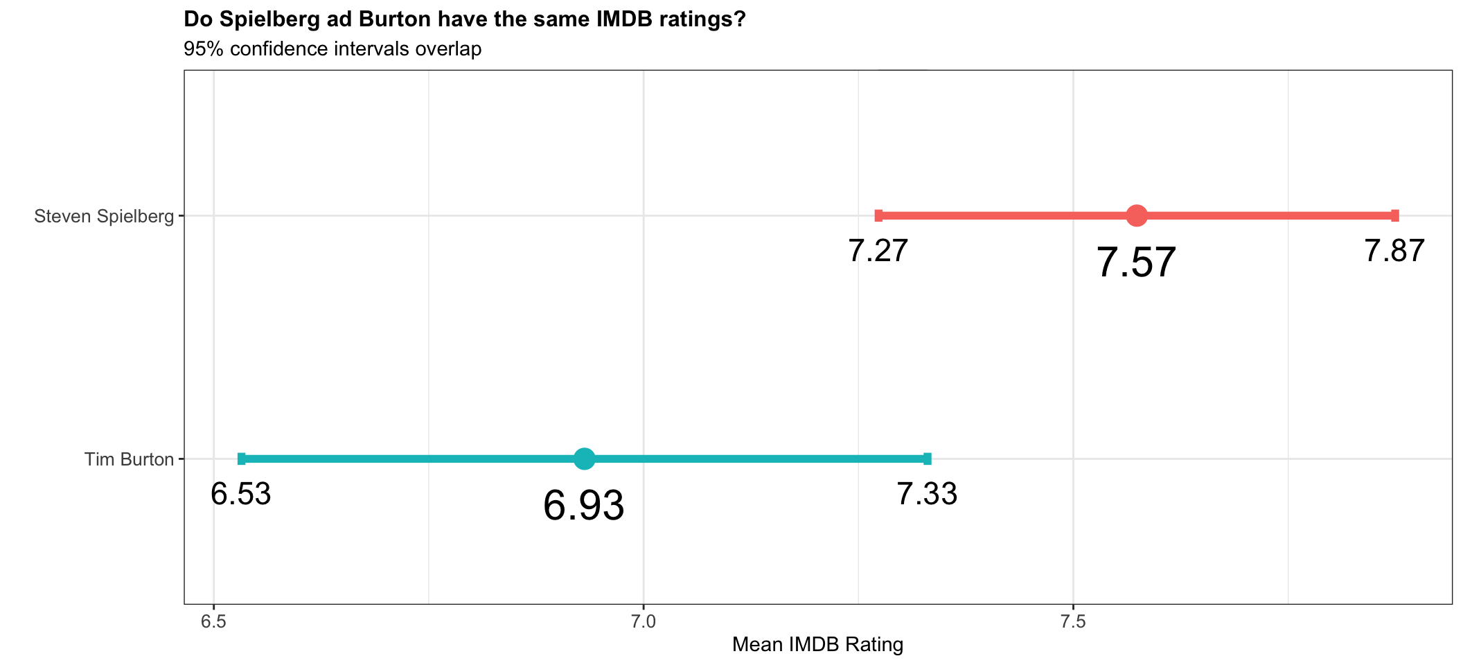
Hypothesis Testing: Null Hypothesis H0: Difference of avergae ratings of Spielberg and Burton equals 0 Alternative Hypothesis H1: Difference in Means not equal to 0.
testrating <- movies %>%
  filter(director %in% c("Steven Spielberg", "Tim Burton")) %>%
  select(director, rating)

t.test(testrating$rating ~ testrating$director)
##
## Welch Two Sample t-test
##
## data: testrating$rating by testrating$director
## t = 2.7144, df = 30.812, p-value = 0.01078
## alternative hypothesis: true difference in means between group Steven Spielberg and group Tim Burton is not equal to 0
## 95 percent confidence interval:
## 0.1596624 1.1256637
## sample estimates:
## mean in group Steven Spielberg mean in group Tim Burton
## 7.573913 6.931250We test the difference between means of the two directors, and the t-stat value equals 3 while the p-value is 0.01. The confidence interval is [0.16,1.13] and does not contain the value 0. The t-statistics value is greater than 2, p-value < 5% and 0 lies outside the confidence interval, therefore we reject H0.
obs_diff1 <- testrating %>%
  specify(rating ~ director) %>%
  calculate(stat = "diff in means", order = c("Steven Spielberg", "Tim Burton"))
obs_diff1
## Response: rating (numeric)
## Explanatory: director (factor)
## # A tibble: 1 x 1
## stat
## <dbl>
## 1 0.643null_dist1 <- testrating %>%
# specify variables
specify(rating ~ director) %>%
# assume independence, i.e, there is no difference
hypothesize(null = "independence") %>%
# generate 1000 reps, of type "permute"
generate(reps = 1000, type = "permute") %>%
# calculate statistic of difference, namely "diff in means"
calculate(stat = "diff in means", order = c("Steven Spielberg", "Tim Burton"))
null_dist1## Response: rating (numeric)
## Explanatory: director (factor)
## Null Hypothesis: independence
## # A tibble: 1,000 x 2
## replicate stat
## <int> <dbl>
## 1 1 0.0492
## 2 2 -0.491
## 3 3 -0.110
## 4 4 -0.332
## 5 5 -0.290
## 6 6 0.282
## 7 7 0.272
## 8 8 -0.290
## 9 9 -0.237
## 10 10 0.0174
## # … with 990 more rowsggplot(data = null_dist1, aes(x = stat)) +
geom_histogram()+
theme_bw()## `stat_bin()` using `bins = 30`. Pick better value with `binwidth`.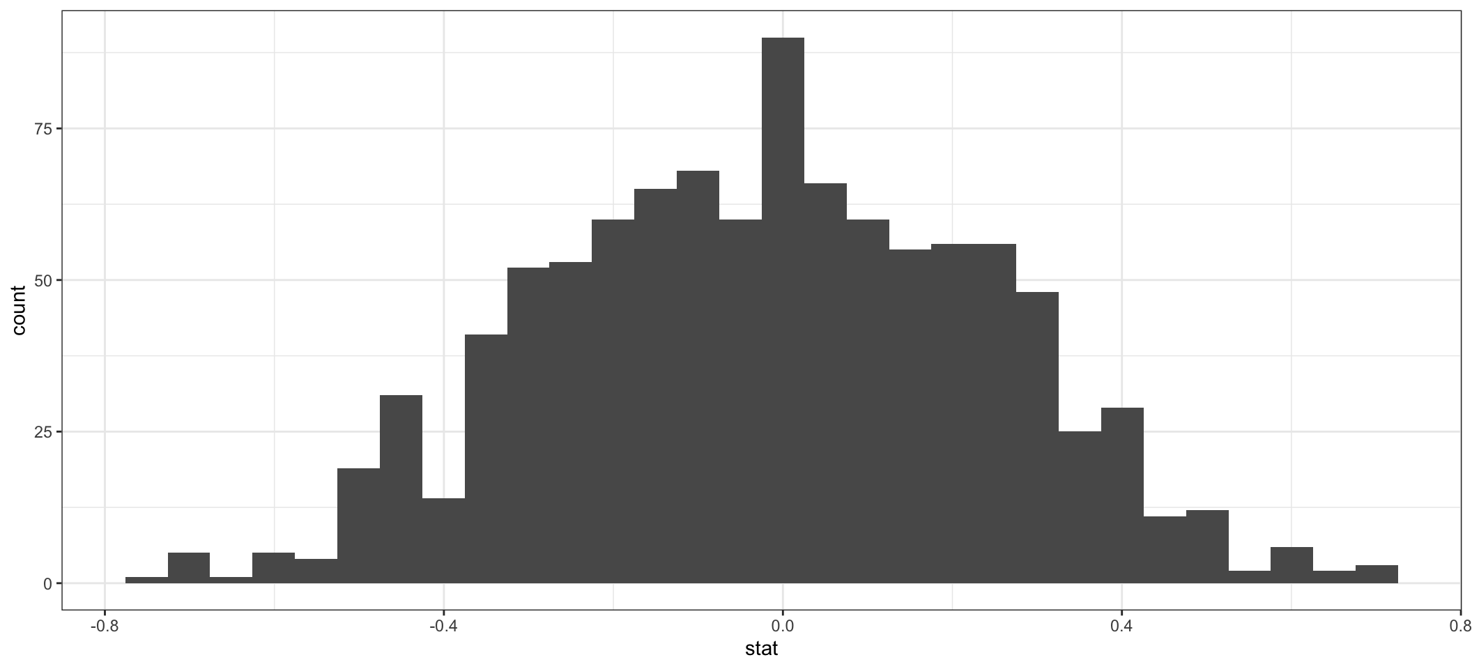
obs_stat1 <- obs_diff1 %>% pull() %>% round(2)
obs_stat1
## [1] 0.64null_dist1 %>% visualize() +
shade_p_value(obs_stat = obs_diff1, direction = "two-sided")+
theme_bw()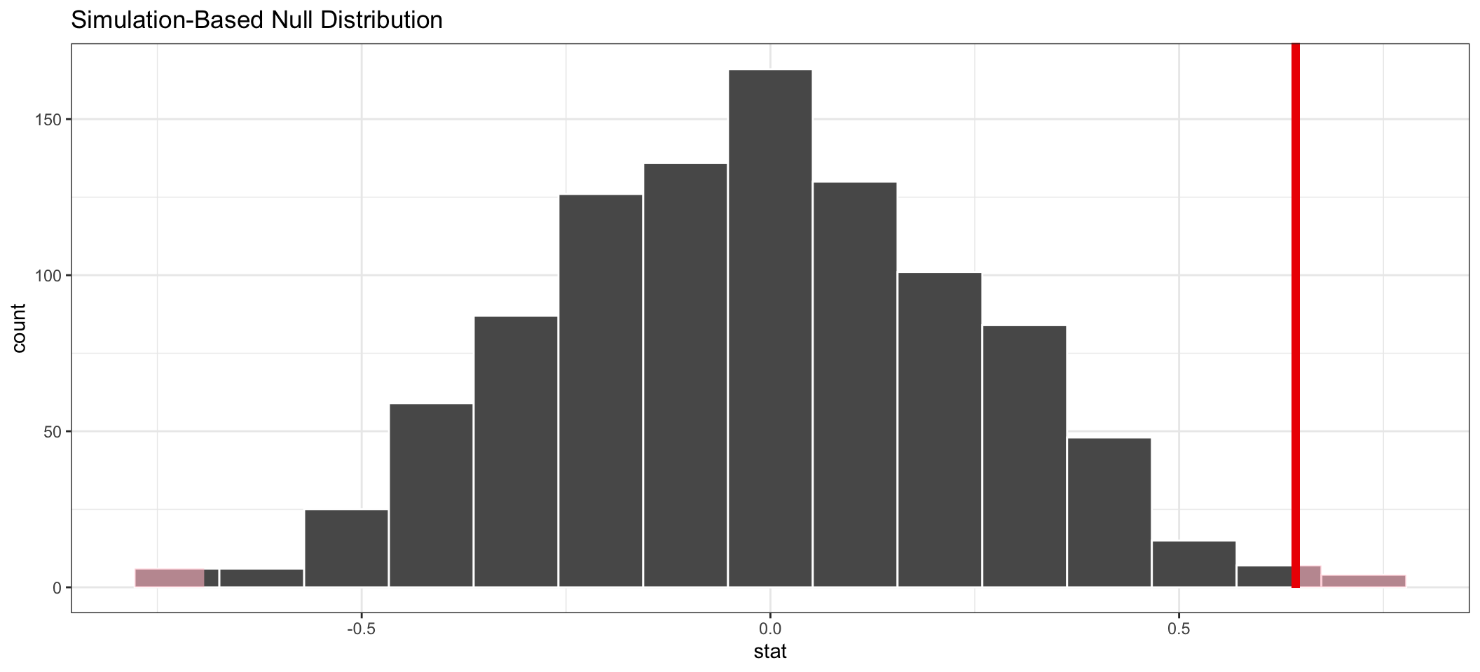
null_dist1 %>%
  get_p_value(obs_stat = obs_diff1, direction = "two_sided")
## # A tibble: 1 x 1
## p_value
## <dbl>
## 1 0.008